German Flower of the Year 2023: The Small Self-Heal

Flower of the Year
The Loki Schmidt Foundation has chosen the Small Self-Heal (Prunella vulgaris) as the Flower of the Year 2023 to draw attention to the gradual loss of numerous plant and animal species. The Small Self-Heal grows between 5 and 25 cm tall and delights observers with its small, violet flowers. Despite its delicate appearance, it thrives in frequently mowed lawns and tolerates grazing and trampling by livestock. Despite its robustness, this once common wildflower shares the fate of many other species found in meadows, pastures, and roadsides: its populations are steadily declining.

Allowing More Wilderness

The gradual loss of species is particularly evident in the case of the once common Small Self-Heal. It can thrive in many places, as long as they are not too nutrient-rich. When meadows, pastures, and paths are fertilized or surrounding landscapes are over-fertilized, it significantly impacts the composition of plant communities: a few fast-growing plant species that grow tall and dense tend to overgrow the diverse, formerly lean habitats. Currently, the Small Self-Heal is present in all federal states and is not at risk everywhere. However, in some regions of Germany, a decline in populations is noticeable, such as in Mecklenburg-Western Pomerania, Brandenburg, Hesse, Baden-Württemberg, and Bavaria.

A New Badge for You!

If you find and identify a Small Self-Heal, you will be rewarded with a new badge for your profile: the Flower of the Year 2023.

This article was featured in the Flora-Incognita app as a story in the summer of 2023. The app provides intriguing information about plants, ecology, species identification, as well as tips and tricks for plant identification. Why not take a look?

Heterophylly: One Plant – Different Leaves

The leaves of a plant are often a crucial feature for species identification: the leaf of the Wych Elm (Ulmus glabra) has a serrated edge, the leaves of the Wild Tulip (Tulipa sylvestris) are soft and hairless, and the leaves of the Guelder Rose (Viburnum opulus) are always arranged oppositely. There are many examples of plants whose leaves look so unmistakably that the corresponding species can be confidently identified. However, this does not apply to all plants! Some species respond to environmental influences by changing certain characteristics of their leaf shape, such as the size of the leaf surface or the density of leaf venation.

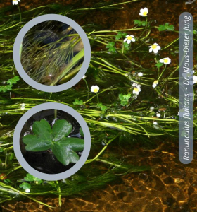
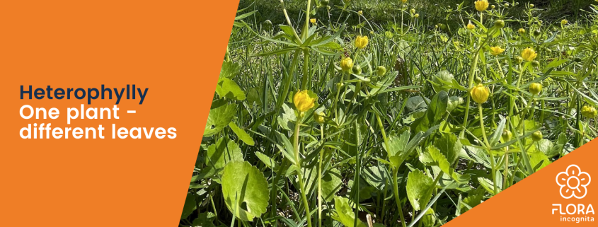
“Leaf polymorphism” (heterophylly) means that a single plant can have very differently shaped leaves. Some herbs can produce several very different leaf forms, so distinct that they might not be attributed to the same species. A notable example of this is found in some species of the genus Ranunculus, commonly known as buttercups. For instance, the Water Buttercup (genus Ranunculus, section Batrachium) has two completely different leaf forms: the finely divided leaves underwater (submerged leaves) and the roughly three-parted dissected leaves that float (floating leaves).

To understand the phenomenon of heterophylly, one must consider the genetics of the plant. The Water Buttercup has a genotype, a genetic basis for its plant traits, but two different leaf phenotypes (physical appearances). Through years of research, even at the molecular genetic level, scientists have determined which genes need to be activated to initiate the formation of a specific leaf shape. The role of plant growth hormones, their concentrations, and flows that determine the final leaf shape has also been investigated. In the case of the Water Buttercup, the pronounced leaf polymorphism is an adaptation to the environment.

However, there are also examples of leaf polymorphism that remain mysterious to this day, as they cannot be explained by environmental adaptations. Among the early spring plants that push their leaves out of the ground, there is the Goldilocks Buttercup (Ranunculus auricomus agg.). What sets this group of species apart is that the same plant can produce completely different leaf forms, depending on whether it has just emerged from winter dormancy, whether it is flowering, or fruiting.

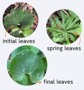
Within a plant individual, an entire leaf cycle occurs, starting with relatively small and simply three-parted leaves (initial leaves) that emerge immediately after winter. Around April, when the plant starts to bloom, more or less deeply divided leaf forms appear, typically used for species identification. Later in the year, when the plant is fruiting, less dissected leaf forms reappear (summer leaves, final leaves). These resemble the initial leaves but are larger. Why the Goldilocks Buttercup exhibits such leaf diversity within a year remains unclear. An adaptation to the environment, as in the case of the Water Buttercup, could not be demonstrated here.

What remains a puzzle for plant development poses a real challenge for botanical systematists. How can one reasonably morphologically define a plant species like the Goldilocks Buttercup when it constantly changes throughout the year? A tough nut to crack (and a subject of ongoing refinement) even for Flora Incognita!

This article was featured in the Flora-Incognita app as a story in the summer of 2023. The app provides intriguing information about plants, ecology, species identification, as well as tips and tricks for plant identification. Why not take a look?

How to export your Flora Incognita records to a custom map (Google Maps, QGIS and R)

We get asked quite often of whether one can view the personal plant observations outside of the Flora Incognita app, for example in Google Maps or a Geographic Information System (GIS). The answer is simple: Yes, you can! In this article, you will find three tutorials for that – depending on your use case.

Exporting your data out of Flora Incognita

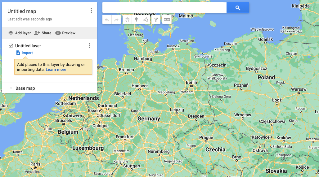
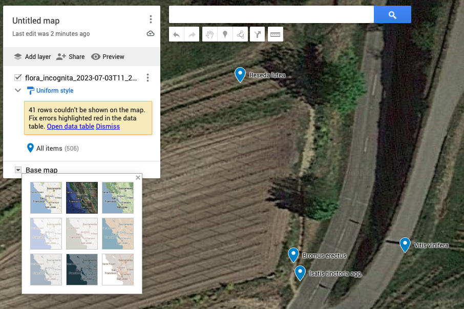
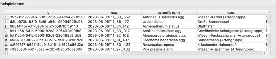
Regardless of the method you choose, first, you need to export your observations from the Flora Incognita app. To do that:

1) Open your observation list under My Observations from the home screen and tap on the Share icon at the top right.

2) You can now transfer either a .csv file or a .gpx file to your computer using various methods.

3) If you want to export your observations including the images, we recommend that you first filter the observation list to reduce the number of observations to be exported. The reason for this is the enormous increase in file size caused by the images.


Exporting Flora Incognita observations to Google Maps

With this method, you can view your findings in Google Maps on the desktop without requiring any additional software.

  1. Go to https://www.google.com/intl/en/maps/about/mymaps/ and start a new project under Get Started.
  2. Click on the Owned tab and select Create a New Map. You will get a blank map with its own context menu:
  3. Under Untitled Layer, click on Import and choose the previously exported .csv file.
  4. In the following menu, select the latitude and longitude columns. Click Continue.
  5. Now choose how your data points should be labeled. Choose name for the common name or scientific name for the scientific name. Click Finish. Note: The points are now marked but the labels are not visible yet.
  6. In the menu window, click on Uniform Style and choose the name you want to display under Label.
  7. Under Base Map, you can customize the underlying map as desired:
  8. Further individual adjustments are possible under the available menu options. Clicking on a data point will display the transferred meta-information.

Exporting Flora Incognita observations to QGIS

QGIS is a professional GIS application developed based on Free and Open-Source Software (FOSS). Choosing this option is useful if you work professionally or in your free time with GIS.

  1. Open QGIS and create a new project (Project -> New).
  2. In the left menu, select your map base layer under XYZ Tiles by double-clicking. In our example, we use OpenStreetMap. You can now zoom into the map.
  3. In the main navigation, select Layer -> Add Layer -> Add Delimited Text Layer.
  4. Choose your previously exported .csv file and check the extracted file format for the following parameters:
    • File format: CSV (comma separated values)
    • Geometry definition: X field: longitude; Y field: latitude
    • Geometry: EPSG:4326 – WGS 84

    Your data should look like this:

  5. Click Add at the bottom right and close the window. Now you will see your discoveries in the map, but still without labels. Learning how to customize your findings is the next step.
  6. Right-click on your Flora Incognita layer in the Layer panel to the left of the map. Select Properties.
  7. Under Label change the setting from No Label to Single Label. Under Value you can choose whether you want to display the scientific or the trivial name. Confirm with OK. The result looks like this:

Exporting Flora Incognita observations with R

R is a free programming language for statistical calculations and graphics. To follow this guide, you need to execute prepared scripts using the appropriate software. Basic knowledge of R is required.

  1. Go to https://www.r-project.org and install the latest version of the R program.
  2. Go to https://posit.co/products/open-source/rstudio/ and install the latest RStudio.
  3. Install and load the necessary libraries.

    install.packages("leaflet")
    install.packages("leaflet.extras2")
    install.packages("htmlwidgets")


    library(leaflet)
    library(leaflet.extras2)
    library(htmlwidgets)
  1. Read your .csv file.

    dat<-read.csv("/your/path/your_file.csv", header=TRUE)
  1. Create and load the map. Closely located observations are clustered.

    map1 %
    addProviderTiles('OpenStreetMap.Mapnik') %>%
    addCircleMarkers(lng = ~longitude, lat = ~latitude,
    label = ~scientific.name, radius=7, labelOptions = labelOptions(style = list("color" = "black"),
    noHide = T, textOnly=T, textsize = "10px", offset = c(1, 12)),
    color="black", clusterOptions = markerClusterOptions(spiderfyOnMaxZoom=T))

    map1
  1. Add the plant findings to the map. To display the trivial name, replace “scientific.name” with “name”.

    map2 %
    addProviderTiles('OpenStreetMap.Mapnik') %>%
    addLabelOnlyMarkers(lng = ~longitude, lat = ~latitude, group="labs",
    label = ~scientific.name, labelOptions = labelOptions(style = list("color" = "black"),
    noHide = T, textOnly=T, textsize = "10px", offset = c(1, 12))) %>%
    addCircleMarkers(lng = ~longitude, lat = ~latitude, color="black") %>%
    addCircleMarkers(lng = ~longitude, lat = ~latitude, radius=2, label = ~scientific.name, color="white")
    addLabelgun(map2, group="labs")

    map2
  1. Export your map as an .html file
    saveWidget(map2, file="/yourpath/map.html")

    Screenshot from the map generated with R. Three plant findings are visible in a lake landscape.

You can also download the guide as a text file: R_MapExport_EN