How to export your Flora Incognita records to a custom map (OpenStreetMap, QGIS, R and Google)
We get asked quite often of whether one can view the personal plant observations outside of the Flora Incognita app, for example in Google Maps or a Geographic Information System (GIS). The answer is simple: Yes, you can! In this article, you will find three tutorials for that – depending on your use case.
Exporting your data out of Flora Incognita
 Regardless of the method you choose, first, you need to export your observations from the Flora Incognita app. To do that:
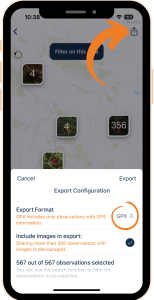
1) Open your observation list under My Observations from the home screen and tap on the Share icon at the top right.
2) You can now transfer either a .csv file or a .gpx file to your computer using various methods.
3) If you want to export your observations including the images, we recommend that you first filter the observation list to reduce the number of observations to be exported. The reason for this is the enormous increase in file size caused by the images.
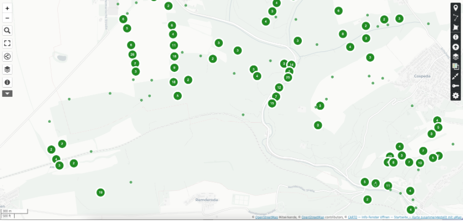
Import Flora Incognita observations as a layer in OpenStreetMap (OSM)
You can use this method to display your observations in OpenStreetMap, display them on your desktop or embed them on your website.
- First, go to uMap (https://umap.openstreetmap.de/en/) to create your map. In this editor you can easily create maps with OpenStreetMap layers (https://www.openstreetmap.org) and customize them to your needs. Some language variants can be chosen in the drop-down menu at the bottom of the page.
- Click the button “Create a map”
- Select the “Import data” button in the right sidebar
- In the “Import data” menu under “Select files”, select the previously exported file and click on the turquoise “Import data” button at the bottom.
- In the following view, all exported observations are displayed with a standard symbol. This view can now be customized as desired. By using Shift + Command + Click on one of the standard symbols, the properties of all symbols can be changed at once.
- A nice representation as colored, semi-transparent dots can be achieved by first selecting “Circle” under “Shape properties”. The desired transparency can be set using the “Symbol opacity” slider. Using the “Interaction options” -> “Show label” -> “on hover” menu, the name of the species can be displayed as a pop-up when the mouse pointer is hovered over the points.
- The properties of a specific observation (all other columns in the csv file) can be displayed with Shift + Click.
- Observations can be grouped or a heatmap display can be achieved using the “layer type” menu.
- The finished maps can be exported, shared or integrated on a website using the “Share” button on the right-hand side. If necessary, settings can be adjusted under “Options for embedding and for a customized map view” to achieve the desired result.
Exporting Flora Incognita observations to Google Maps
With this method, you can view your findings in Google Maps on the desktop without requiring any additional software.
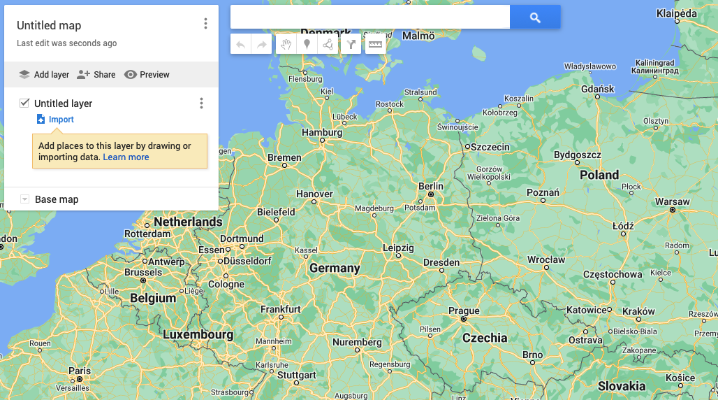
- Go to https://www.google.com/intl/en/maps/about/mymaps/ and start a new project under Get Started.
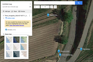
- Click on the Owned tab and select Create a New Map. You will get a blank map with its own context menu:

- Under Untitled Layer, click on Import and choose the previously exported .csv file.
- In the following menu, select the latitude and longitude columns. Click Continue.
- Now choose how your data points should be labeled. Choose name for the common name or scientific name for the scientific name. Click Finish. Note: The points are now marked but the labels are not visible yet.
- In the menu window, click on Uniform Style and choose the name you want to display under Label.
- Under Base Map, you can customize the underlying map as desired:
- Further individual adjustments are possible under the available menu options. Clicking on a data point will display the transferred meta-information.

Exporting Flora Incognita observations to QGIS
QGIS is a professional GIS application developed based on Free and Open-Source Software (FOSS). Choosing this option is useful if you work professionally or in your free time with GIS.
- Open QGIS and create a new project (Project -> New).
- In the left menu, select your map base layer under XYZ Tiles by double-clicking. In our example, we use OpenStreetMap. You can now zoom into the map.
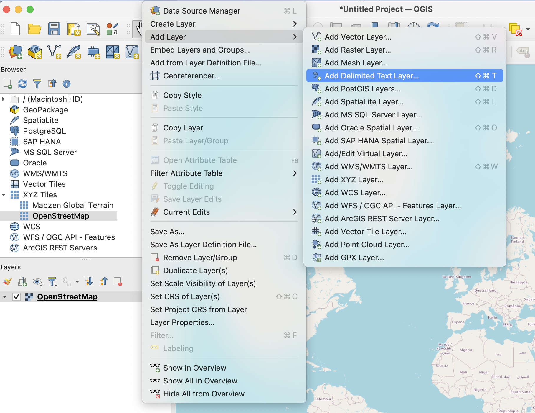
- In the main navigation, select Layer -> Add Layer -> Add Delimited Text Layer.

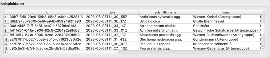
- Choose your previously exported .csv file and check the extracted file format for the following parameters:
- File format: CSV (comma separated values)
- Geometry definition: X field: longitude; Y field: latitude
- Geometry: EPSG:4326 – WGS 84
Your data should look like this:

- Click Add at the bottom right and close the window. Now you will see your discoveries in the map, but still without labels. Learning how to customize your findings is the next step.
- Right-click on your Flora Incognita layer in the Layer panel to the left of the map. Select Properties.
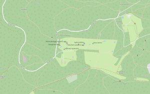
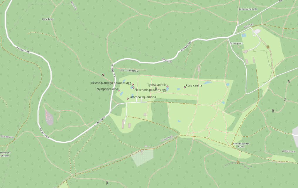
- Under Label change the setting from No Label to Single Label. Under Value you can choose whether you want to display the scientific or the trivial name. Confirm with OK. The result looks like this:
Exporting Flora Incognita observations with R
R is a free programming language for statistical calculations and graphics. To follow this guide, you need to execute prepared scripts using the appropriate software. Basic knowledge of R is required.
- Go to https://www.r-project.org and install the latest version of the R program.
- Go to https://posit.co/products/open-source/rstudio/ and install the latest RStudio.
- Install and load the necessary libraries.
install.packages("leaflet")

install.packages("leaflet.extras2")

install.packages("htmlwidgets")
library(leaflet)

library(leaflet.extras2)

library(htmlwidgets)
- Read your .csv file.
dat<-read.csv("/your/path/your_file.csv", header=TRUE)
- Create and load the map. Closely located observations are clustered.
map1 %

addProviderTiles('OpenStreetMap.Mapnik') %>%

addCircleMarkers(lng = ~longitude, lat = ~latitude,

label = ~scientific.name, radius=7, labelOptions = labelOptions(style = list("color" = "black"),

noHide = T, textOnly=T, textsize = "10px", offset = c(1, 12)),

color="black", clusterOptions = markerClusterOptions(spiderfyOnMaxZoom=T))
map1
- Add the plant findings to the map. To display the trivial name, replace “scientific.name” with “name”.
map2 %

addProviderTiles('OpenStreetMap.Mapnik') %>%

addLabelOnlyMarkers(lng = ~longitude, lat = ~latitude, group="labs",

label = ~scientific.name, labelOptions = labelOptions(style = list("color" = "black"),

noHide = T, textOnly=T, textsize = "10px", offset = c(1, 12))) %>%

addCircleMarkers(lng = ~longitude, lat = ~latitude, color="black") %>%

addCircleMarkers(lng = ~longitude, lat = ~latitude, radius=2, label = ~scientific.name, color="white")

addLabelgun(map2, group="labs")
map2
- Export your map as an .html file
saveWidget(map2, file="/yourpath/map.html")

You can also download the guide as a text file: R_MapExport_EN
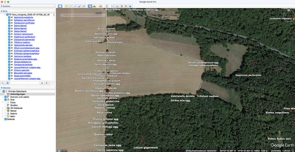
Import Flora Incognita observations as a layer in Google Earth Pro
With this method you can display your plant observations in Google Earth, show them on your desktop or embed them on your website.
- First, you need to download Google Earth Pro (desktop or mobile version).
- Open the program and click File -> Import
- Select the previously exported file with “Open” and set “Comma” as the separator. Click on “Next” and make sure that “latitude” is entered in the “Latitude” field and ‘longitude’ in the “Longitude” field. Then click on “Finish”.
- Answer the following question “Do you want to apply a style sheet to the imported elements?” with ”Yes”
- The display format of the observations can be adjusted in the tabs that now appear. If the species name is to be displayed in the map, you can select “name” or “scientific name” in the name field, for example. The color and the symbol to be used can also be selected in the subsequent tabs.
- In the left-hand column under “Places”, the imported map layer can now be selected and, if necessary, individual observations can be deactivated.
- Left-click on an observation to display all other associated columns from the csv table and right-click on the observation to add further information or images to an observation, for example.
- The created map layer can then be saved under File -> Save -> My Places.